Eduki

Summarizing categorical data using a frequency table

Categorical data only take categories as values and can be well-represented using frequency tables. Below is a frequency distribution table that shows the distribution of dog breeds. On the right is the relative frequency distribution table, where the occurrence of each value is expressed as the percentage of the total number of occurrences. 

[Data to Frequency table]

Summarizing categorical data using a bar diagram

We often represent the distribution of categorical data using a bar graph, which simply shows the frequencies of categories in a graphical form.  A bar graph also uses a horizontal line. Above it, we draw a rectangle (or “bar”) to represent each category in the data set. The height of a bar tells us the frequency of the category. There are 12 German shepherds in the data set, so the bar for this category is 12 units tall. Below the line, we write the labels for the categories. In a bar graph, however, the categories can be listed in any order. The bar that shows the frequency of pugs can be placed anywhere along the horizontal line. 

Frequency table and bar diagram]

Bar diagram vs Histogram 

Bar graphs and histograms may seem alike, but they are very different. Unlike a histogram which summarizes numerical data, a bar diagram is used to represent categorical data.

Here is a bar graph showing the breeds of 30 dogs and a histogram for their weights.

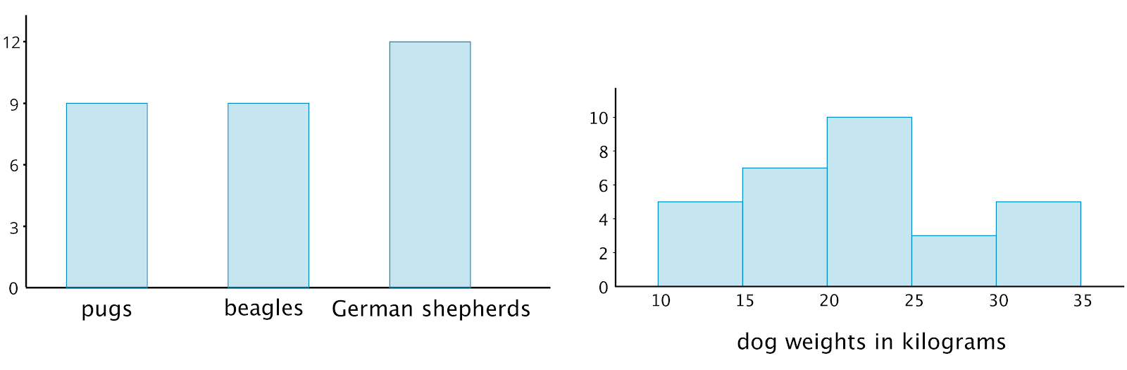
So, how are they different?

1. Bar graphs represent categorical data. Histograms represent numerical data. 

2. Bar graphs have spaces between the bars to separate categories. Histograms show a space between bars only when no data values fall between the bars.

3. Bars in a bar graph can be in any order. Histograms must be in numerical order.

4. In a bar graph, the number of bars depends on the number of categories. In a histogram, we choose how many bars to use.

Mode as the typical value of a categorical distribution

A bar diagram is useful for identifying important features of the distribution of the data. Since the categories have no natural order and their arrangement could change, the idea of the center of the distribution does not make much sense for categorical data such as these. Instead, the most frequent response is often reported and used as a representative or “typical” value for the data. This quantity is called the mode or the modal category.

[Bar diagram]

The mode is the only method of describing a “typical” value for categorical data. In our example above, the category “German Shepherd” is the mode or the modal category. Keep in mind that mode refers to the category that occurred the most, rather than the frequency of that category. So, in our example, the most frequent value is “German Shepherd” which occurs 12 times. The mode here is “German Shepherd” and its frequency is 12. It is incorrect to say that the mode of the data is 12. 

Can a distribution have multiple modes?

It is not uncommon for categorical data to have multiple modes. For example, if your survey led to your classmates having 12 German Shepherds and 12 Golden Retrievers, then the resulting data would have two modes - “German Shepherd” and “Golden Retriever”. It is also possible to have more than two modes. In the extreme case when the data is evenly distributed, i.e. the frequency of all the categories is the same, all categories (or none of the categories) can be considered the mode. 

[bar diagrams here]